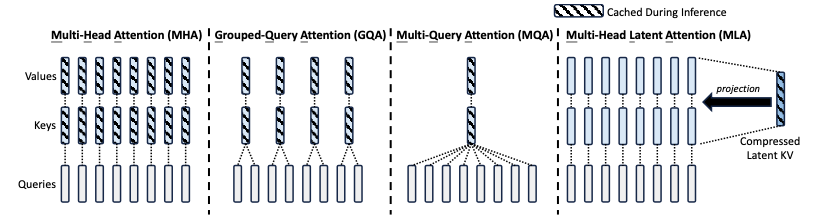
Autoregressive language models based on the decoder-only Transformer architecture generate tokens sequentially, conditioning each prediction on all previously generated tokens. During inference, the key-value pairs of prior tokens must be retained to ensure coherence across the generation sequence. In the standard Multi-Head Attention (MHA) formulation, the size of this KV cache grows linearly with both the sequence length and the number of attention heads, creating a significant memory bottleneck that limits the maximum context length achievable on commodity hardware. Multi-Head Latent Attention (MLA), introduced in DeepSeek-V2, addresses this bottleneck through low-rank joint projection of the key and value representations, achieving KV cache sizes comparable to Grouped-Query Attention (GQA) while preserving — and in some cases exceeding — the modeling capacity of full MHA.

This article presents a detailed analysis of the MLA mechanism, including its low-rank compression strategy, the decoupled Rotary Position Embedding (RoPE) design, and the weight-absorption trick that enables efficient inference. We also provide a rigorous comparison of the computational and memory costs of MLA relative to MHA, MQA, and GQA.

Notation

Background: KV Cache in Autoregressive Transformers

In a decoder-only Transformer, each autoregressive step processes the current token embedding $h_t$ through a series of projections to produce query, key, and value vectors for every attention head:

where $W_Q, W_K, W_V \in \mathbb{R}^{d_h n_h \times d}$ are the projection weight matrices and $q_{t,i}, k_{t,i}, v_{t,i} \in \mathbb{R}^{d_h}$ denote the query, key, and value for head $i$ of token $t$.

Within each head, the attention output is computed as a weighted sum over all prior values:

The final layer output is obtained by concatenating the per-head outputs and projecting:

To avoid redundant recomputation, the key-value pairs $(k_{j,i}, v_{j,i})$ are cached after their first computation. The per-token KV cache size in MHA is therefore $2 \, n_h \, d_h$ per layer, yielding a total cache of $2 \, n_h \, d_h \, l$ elements per token. For a model with $n_h = 64$, $d_h = 128$, and $l = 60$, this amounts to nearly one million float16 parameters per token — a substantial memory footprint that grows without bound as the sequence length increases.

Prior Approaches: MQA and GQA

Multi-Query Attention (MQA) [Shazeer, 2019] collapses all heads to share a single pair of key and value projections, reducing the per-token KV cache to $2 \, d_h \, l$. Although effective in reducing memory, the aggressive sharing of KV representations across heads degrades model quality, as each head loses its distinctive key-value subspace.

Grouped-Query Attention (GQA) [Ainslie et al., 2023] interpolates between MHA and MQA by partitioning the $n_h$ query heads into $n_g$ groups, each sharing one key-value head. The per-token KV cache becomes $2 \, n_g \, d_h \, l$, where $n_g$ controls the trade-off between cache efficiency and model capacity. When $n_g = n_h$, GQA reduces to MHA; when $n_g = 1$, it reduces to MQA.

Complexity Comparison

It is instructive to compare the per-token KV cache and the per-layer FLOPs for each attention variant. For a sequence of length $T$ with hidden dimension $d = n_h d_h$:

In MHA, the KV projection matrices $W_K, W_V \in \mathbb{R}^{n_h d_h \times d}$ require $2 n_h d_h d$ FLOPs per token, and the cache must store $2 n_h d_h$ elements per layer. GQA reduces the projection cost to $2 n_g d_h d$ by sharing KV within each group, but the cache reduction is proportional to $n_g / n_h$. MQA achieves the smallest projection cost of $2 d_h d$ but at the cost of collapsing all head-specific information. MLA, by contrast, uses a single compressed vector of dimension $d_c \ll n_h d_h$ from which both key and value are up-projected. The key and value projection costs are each $d_c \cdot d$, and the cache stores only $d_c + d_h^R$ elements (the compressed vector plus the decoupled RoPE key). Critically, the cache size is independent of $n_h$, which allows MLA to increase the number of heads freely without any cache penalty — a property that none of the other methods possess.

Low-Rank Joint Key-Value Compression

The central innovation of MLA is the joint low-rank compression of the key and value representations. Rather than projecting $h_t$ independently into key and value spaces of dimension $n_h d_h$, MLA first projects it into a low-dimensional latent space and then up-projects separately to recover the key and value:

Here $c_t^{KV} \in \mathbb{R}^{d_c}$ is the compressed latent vector, which is the only representation stored in the KV cache during inference. The down-projection matrix is $W_{DKV} \in \mathbb{R}^{d_c \times d}$, and the up-projection matrices are $W_{UK} \in \mathbb{R}^{n_h d_h \times d_c}$ and $W_{UV} \in \mathbb{R}^{n_h d_h \times d_c}$. The compression dimension $d_c$ is chosen to be much smaller than $n_h d_h$; in DeepSeek-V2, $d_c = 4 d_h$, which for $d_h = 128$ yields $d_c = 512$, compared to $n_h d_h = 8192$ for $n_h = 64$.

The low-rank structure imposes a bottleneck: the key and value vectors for all heads are constrained to lie in a $d_c$-dimensional subspace. This is a form of information compression, and the key question is whether $d_c$ dimensions suffice to preserve the expressive power of the full-rank key and value. Empirically, DeepSeek-V2 demonstrates that with $d_c = 4 d_h$, MLA not only matches but slightly exceeds the performance of MHA — a result we revisit in the discussion of experimental results.

To further reduce the memory footprint during training (where the query activations must also be stored for backpropagation), MLA applies the same low-rank compression strategy to the query:

where $c_t^Q \in \mathbb{R}^{d_c'}$ is the compressed query latent, $W_{DQ} \in \mathbb{R}^{d_c' \times d}$, and $W_{UQ} \in \mathbb{R}^{n_h d_h \times d_c'}$. Note that the query compression affects only training memory, not inference cache size, since queries are not cached.

Decoupled Rotary Position Embedding

Rotary Position Embedding (RoPE) [Su et al., 2024] encodes positional information by applying a rotation matrix to the query and key vectors. For a vector $x \in \mathbb{R}^{2m}$, the rotation at position $t$ is defined as:

where each $R_i^{t} \in \mathbb{R}^{2 \times 2}$ is a 2D rotation by angle $t \theta_i$:

The key property of RoPE is that the attention score between a query at position $t$ and a key at position $s$ depends only on the relative position $t - s$:

since $R(t)^\top R(s) = R(s - t)$ by the group structure of rotation matrices.

The Incompatibility Problem

In MLA, the key is reconstructed from the compressed latent: $k_t^C = W_{UK} \, c_t^{KV}$. If one were to apply RoPE naively by rotating the reconstructed key, the result would be $R(t) \, W_{UK} \, c_t^{KV}$. Since $c_t^{KV}$ is the cached quantity, this rotation must be applied at every inference step for all cached positions — defeating the purpose of caching. Moreover, the rotation matrix $R(t)$ cannot be absorbed into $W_{UK}$ because $R(t)$ is position-dependent and varies across tokens; there is no fixed matrix that can be pre-multiplied into $W_{UK}$ to account for all positions simultaneously.

Equivalently, consider attempting to absorb $R(t)$ into $W_{UK}$. We would like to write:

but $\tilde{W}_{UK}(t)$ depends on the position $t$, meaning it cannot be pre-computed and must be materialized for each token — incurring an $O(d_c \cdot n_h d_h)$ cost per token, which is exactly the cost we sought to avoid.

The Decoupled Solution

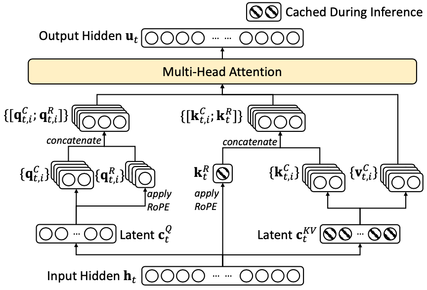
DeepSeek-V2 resolves this by separating the positional and content components of the key. The content information is carried by the compressed latent $c_t^{KV}$ (up-projected without RoPE), while the positional information is carried by a separate, small set of RoPE-encoded key vectors that are shared across all heads.

Query side. The compressed query latent $c_t^Q$ is first up-projected and then RoPE is applied:

where $W_{QR} \in \mathbb{R}^{n_h d_h^R \times d_c'}$ produces a separate set of RoPE queries of dimension $d_h^R$ per head. The final query for head $i$ is the concatenation of the content and positional parts:

Key side. The content key is up-projected from the compressed latent without RoPE:

and the positional key is produced from the raw hidden state with RoPE:

where $W_{KR} \in \mathbb{R}^{d_h^R \times d}$ and the resulting $k_t^R$ is shared across all heads. The final key for head $i$ is:

This decoupling ensures that the compressed latent $c_t^{KV}$ is stored as-is in the cache (without any position-dependent transformation), while the position information is captured by the small additional vector $k_t^R$ of dimension $d_h^R$.

Attention Score Computation

With the decoupled query and key, the attention score for head $i$ decomposes into a content component and a positional component:

The attention output is then:

The per-token cache now stores $c_j^{KV} \in \mathbb{R}^{d_c}$ and $k_j^R \in \mathbb{R}^{d_h^R}$, for a total of $d_c + d_h^R$ elements per layer — independent of $n_h$.

Inference-Time Weight Absorption

A crucial advantage of MLA is that the up-projection matrices $W_{UK}$ and $W_{UV}$ can be absorbed into other weight matrices at inference time, effectively eliminating the cost of explicitly reconstructing the full key and value vectors.

Key Absorption: $W_{UK}$ into $W_Q$

Consider the content term of the attention score:

where $W_{UQ,i}, W_{UK,i} \in \mathbb{R}^{d_h \times d_c'}$ and $\mathbb{R}^{d_h \times d_c}$ respectively are the slices of the up-projection matrices corresponding to head $i$. The product $W_{UQ,i}^\top W_{UK,i} \in \mathbb{R}^{d_c' \times d_c}$ can be pre-computed once and reused for all tokens, since it depends only on the model weights, not on the input. Let us define:

Then the content attention score simplifies to:

This means the attention score is computed directly from the compressed representations $c_t^Q$ and $c_j^{KV}$, without ever materializing the full $d_h$-dimensional key or query vectors. The pre-computed matrix $\hat{W}_{QK,i}$ has size $d_c' \times d_c$, which is small compared to the original key projection $W_{UK,i} \in \mathbb{R}^{d_h \times d_c}$.

Value Absorption: $W_{UV}$ into $W_O$

After computing the attention weights, the weighted sum of values is:

where $\alpha_{t,j,i}$ are the attention weights for head $i$ and $W_{UV,i} \in \mathbb{R}^{d_h \times d_c}$ is the value up-projection for head $i$. Since the weighted sum $\sum_j \alpha_{t,j,i} \, c_j^{KV}$ is a vector in $\mathbb{R}^{d_c}$, the computation proceeds as:

1. Compute the weighted sum in the compressed space: $\hat{c}_t^{KV,i} = \sum_j \alpha_{t,j,i} \, c_j^{KV} \in \mathbb{R}^{d_c}$.
2. Up-project: $o_{t,i} = W_{UV,i} \, \hat{c}_t^{KV,i}$.

Now, the final output projection concatenates all heads and applies $W_O$:

This can be rewritten by merging $W_O$ and $W_{UV}$ into a single matrix. Let $W_O = [W_{O,1}, \ldots, W_{O,n_h}]$ where $W_{O,i} \in \mathbb{R}^{d \times d_h}$. Then:

where $\hat{W}_{OV,i} = W_{O,i} \, W_{UV,i} \in \mathbb{R}^{d \times d_c}$ can be pre-computed. The net effect is that the value up-projection and output projection are fused into a single $d \times d_c$ matrix multiplication per head, and the full $d_h$-dimensional value vectors never need to be materialized.

Summary of Absorption Benefits

The absorption trick transforms MLA from a method that merely compresses the cache into one that also reduces the computational cost of the attention operation itself.

Experimental Results

The following table summarizes the per-token KV cache comparison across methods, using the DeepSeek-V2 configuration where $d_c = 4 d_h$ and $d_h^R = d_h / 2$:

For $n_h = 64$ and $d_h = 128$, MHA requires $16384$ elements per layer per token, while MLA requires only $576$ — a compression ratio of approximately $28.4\times$.

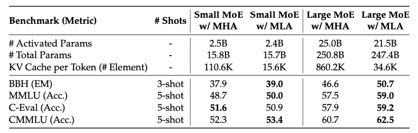
The benchmark results demonstrate that MLA not only matches but slightly exceeds MHA across a range of evaluation metrics. This may appear counterintuitive for a compression-based method, but the explanation lies in the architectural flexibility afforded by the independence of the KV cache from the head count. In standard MHA, increasing the number of heads linearly increases the KV cache, creating a hard constraint on model width. In MLA, the KV cache size depends only on $d_c$ and $d_h^R$, so the number of heads can be increased freely to enhance model capacity without any cache penalty. DeepSeek-V2 exploits this by using approximately $3\times$ the typical head count, distributing the same total hidden dimension across more heads with smaller per-head dimensions. The resulting model has finer-grained attention patterns while maintaining an efficient cache footprint.

References

1. DeepSeek-AI. “DeepSeek-V2: A Strong, Economical, and Efficient Mixture-of-Experts Language Model.” arXiv preprint arXiv:2405.04434, 2024.

2. Shazeer, N. “Fast Transformer Decoding: One Write-Head is All You Need.” arXiv preprint arXiv:1911.02150, 2019.

3. Ainslie, J., Lemercier, P., et al. “GQA: Training Generalized Multi-Query Transformer Models from Multi-Head Checkpoints.” Proceedings of EMNLP, 2023.

4. Su, J., Ahmed, M., Lu, Y., Pan, S., Bo, W., and Liu, Y. “RoFormer: Enhanced Transformer with Rotary Position Embedding.” Neurocomputing, 2024.